Defining the Dominance Axis of the 3D Emotional Model for Expressive Human Audio Emotion

by Simon Lui

Audio emotion research is useful for many different applications. It can be used, for example, to understand the emotion of the speaker on the other end of a phone conversation, to review and improve singers’ performance technique by visualizing their expressive performance, to reproduce emotional musical performance from recording (Lui, Horner and So 2010) or to perform semantic music searches according to information extracted directly from an audio file, etc. Speech emotion research has been a hot topic in recent years. We are now in the midst of an age of information explosion, yet most information on the topic is still only presented in a text format. For example, the online search engine seeks for text information, social network platforms share information in text format (or pictures and video with text tags), online music stores present music selections according to the text index information. On the other hand, a lot of high-level information is embedded in the text, such as the thankfulness in a speech or the anger in a conversation, which are usually related to emotions. Traditionally, the arousal-valence emotional model by Robert Thayer is widely used for expressing emotion (Thayer 1989).

One problem of Thayer’s model is that only using two axes is not enough to classify among different emotions. For example, it is obvious that “happy” is more positive than “angry”. However it is hard to compare the valence between “disgusting” and “fear”. Also, when comparing “very angry” with “angry”, it is hard to define whether “very” refers to higher energy or enhanced valence. Tuomas Eerola and colleagues used a three-dimensional model to predict the emotional rating of music (Eerola, Lartillot and Toiviainen 2009), whereas Albert Mehrabian proposed the Pleasure, Arousal, Dominance (PAD) emotional state model (Mehrabian 1996). The PAD model has one additional dominance axis on top of Thayer’s model. We assume that the pleasure dimension in the PAD model is equivalent to Thayer’s valence. However, very little work has been done on speech emotion with the PAD model. In this work, we investigate on how to define speech emotion by using the three-dimensional PAD model. The model should have objective and measurable axis values so that it doesn’t require manual input.

Implementation

Data Source

The database of German emotional speech is used for emotion classification (Burkhardt et al. 2005). This database consists of speech clips with seven different emotions, including neutral and the big six emotion set (angry, joy, fear, disgust, bored, sad). Ten professional actors recorded a total of 800 clips, each having a duration of 1–6 seconds.

The Energy Axis

The formula of the energy axis is well proven in many other previous works and it is easy to measure. Tin Lay New and colleagues used energy to classify two groups of emotions (Nwe, Wei and De Silva 2003). In their work, the first group consists of “anger”, “surprise” and “joy”, which refer to high-energy sound clips; the second group consists of “fear”, “disgust” and “sadness”, which refers to low-energy sound clips. He achieved a level of accuracy in classification ranging from 70% to 100%. In our work, we use a widely accepted formula of energy — the summation of the square of root mean square (RMS) amplitude. We measured the average energy relative to the maximum of seven different emotions (Table 1). It is very clear that the majority of “joy” and “angry” emotional clips belong to the high-energy class, while “neutral”, “fear” and “disgust” emotional clips belong to medium-energy class, and “sad” and “bored” emotional clips belong to low-energy class.

Table 1. Relative energy of seven emotions.

The Valence Axis

The valence axis should consist of discrete values. In this work, we worked on negative, neutral and positive valence, for various reasons. Firstly, the energy axis alone should be enough to tell the difference between “very angry” and “angry”. These two emotions shouldn’t have difference in terms of valence and dominance. Secondly, the difference between “angry” and “fear” should be described by the dominance axis, because they show no difference in valence or in energy. However, the valence axis cannot be removed. For example, “angry” and “joy”, as well as the non-big six emotion “excited”, all display high energy and high dominance, while they have negative, positive and neutral valence, respectively. Similarly, “sad”, “sleepy” and “satisfied” all show low energy and low dominance, but have negative, neutral and positive valence, respectively. In this work, we use the LFPC shape to classify among three classes of positive, neutral and negative valence.

The Dominance Axis

We performed a test to prove the existence of the dominance axis by dividing the emotional audio data clips into frames of 32 ms and calculating the 12-bins LFPC accordingly. We then calculated the normalized LFPC as follows, where LFPC(n,k) is the LFPC of the nth frame and the kth bin, and S is the RMS Amplitude:

The relative standard deviation (RSD) of the normalized 2nd–6th LFPC is shown in Table 2. The RSD refers to the standard deviation divided by mean. It shows that the RSD is high for lower dominance emotion. We also measured the RSD of LFPC in another way. We further normalized the LFPC to be bounded by 0 and 1, as follows:

Table 3 shows the RSD of the normalized 2nd–6th LFPC bounded within the range of 0 to 1. It presents a similar trend as that seen in Table 2. From the observations of the two experiments above, we suggest that the dominance axis can be described by the RSD of normalized LFPC. A small RSD refers to very firm and aggressive emotion, while a large RSD refers to high level of hesitation and hence defensive emotion. Finally, Table 4 shows some examples of different dominance.

Table 2. The RSD of the normalized 2nd–6th LFPC.

Table 3. The RSD of the normalized 2nd–6th LFPC bounded within the range of 0 to 1.

Table 4. Example of emotions with different dominance.

Orthogonality of the three axes values

We used the Pearson product-moment correlation coefficient (PCC) to evaluate the orthogonality of the three axes. It is found that the three axis formulas have small positive correlation, but quite independent of each other:

Table 5. Covariance of axis value.

Experiments and Discussion

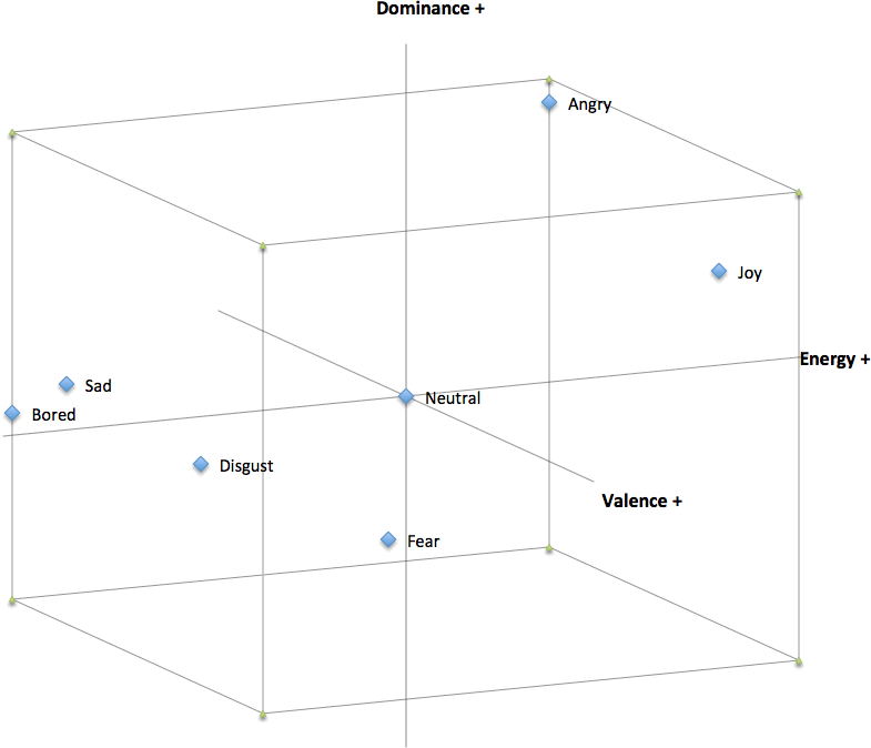
Several experiments were performed to present the identification ability of the proposed three-dimensional emotional model. In the first experiment, we plotted the mean axis values of the seven different emotions we used (Figs. 1–2). The seven emotions can generally be seen to sit quite apart from each other in the model, although sad and bored seem rather close to each other.

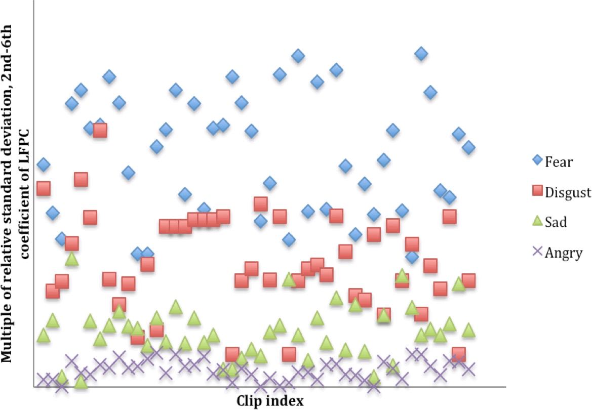
In the second experiment, we demonstrated the emotion identification ability of the dominance axis. We used the product of sequence of the normalized LFPC (LFPC_ps) to calculate the dominance of each sound clip, where LFPC_norm(n,k) is the coefficient of normalized LFPC of the nth frame and the kth bin and where LFPC_ps(p,q) is the product of sequence of the normalized LFPC from bin p to bin q:

The distribution of LFPC_ps(2,6) of 184 negative emotions clips, with 46 clips for each of the angry, fear, disgust and sad emotions, can be seen in Figure 3. The order of average dominance in descending order is fear, disgust, sad, angry. We observed that there are several cases in which the dominance of the “sad” clip is higher than the “fear” clip. This shows that subjective emotional descriptors can scatter in an objective numerical scale. Also, our axis value formula is not finalized; we expect to be able to later narrow down the overlapping area with formula refinement.

In the third experiment, we performed two linear classification tests. The first test runs with a single-class SVM. A linear classification is enough for working with linear axis value. We use SVM to ensure that it is computational efficient with overlapping data. We use a sample size of 46 clips per emotion, for the seven emotions, with each clip having a length of 1–6 seconds. We calculated the average energy, valence and dominance value for each clip in order to generate three-dimensional vector data. Then we set up SVM machines to train the target emotion data against the other six emotions’ data. This is done by a 10-fold cross-validation where 90% of the data is used for training and 10% for testing: it is found that the average accuracy is 85.81% (Table 6). We also performed another a linear classification with k-NN, k=7. The results show an average accuracy of 81.5% (Table 7).

Table 6. 10-fold cross-validation SVM linear classification results.

Table 7. 10-fold cross-validation k-NN (k=7) linear classification result, showing the sample class (left) and the target class (top).

As a comparison, Guven used the same German database and performed speech emotion recognition using SFTF as features and classified with SVM (Guven and Bock 2010). He obtained an average accuracy of 68% in identifying seven emotions. The bottleneck lies on the classifying “disgust” (50% accuracy) and “bored” (60% accuracy). Theodoros Iliou and Christos-Nikolaos Anagnostopoulos used MFCC features and obtained an average accuracy of 94% of identifying seven emotions with neural network (2010), where the speakers are known to the classifier (speaker-dependent). In the case of speaker-independent tests, the overall accuracy is 78% by classifying with SVM, with 55% accuracy for “bored” and 54.5% for “disgust”. In these two works, “disgust” and “bored” are both negative and low-energy emotions. The two emotions can be classified by the third axis in our proposed model effectively. Lugger used 25 audio features, including pitch, formant, harmonic and MFCC. He performed classification with an iterative sequential floating forward selection algorithm (Lugger and Yang 2008), obtaining an average accuracy of 88.8%. However, he only worked on five emotions of the German database. He didn’t work on “disgust” and “fear”; these constitute the main bottleneck for emotion classification.

Future Work

An initial definition of the three continuous axis of the PAD speech emotional model is proposed. This model separates the average value of the seven emotions, with some overlapping among individual samples, since the current axis value formula is not ultimately defined. This initial definition is subject to refinement, as it is not totally orthogonal. We will further refine the definition of the axis formula, in order to reduce the overlapping between different emotions. This work is the first step to approach this final goal. Our ultimate goal is to find a small set of atomic and orthogonal features that can be used to define emotion in a continuous scale model.

Acknowledgements

This work is supported by the SUTD-MIT International Design Center Grant (IDG31200107 / IDD11200105 / IDD61200103).

Bibliography

Burkhardt, Felix, Astrid Paeschke, Miriam Rolfes, Walter F. Sendlmeier and Benjamin Weiss. “A Database of German Emotional Speech,” Interspeech 2005 “Eurospeech”. Proceedings of the 9th European Conference on Speech Communication and Technology (Lisbon: Centro Cultural de Belém, 4–8 September 2005).

Eerola, Tuomas, Olivier Lartillot and Petri Toiviainen. “Prediction of Multidimensional Emotional Ratings in Music from Audio Using Multivariate Regression Models.” ISMIR 2009. Proceedings of the 10th International Society for Music Information Retrieval Conference (Kobe, Japan: International Conference Center, 26–30 October 2009), pp. 621–626.

Guven, Erhan and Peter Bock. “Speech Emotion Recognition using a Backward Context.” AIPR 2010. Proceedings of the 39th Applied Imagery Pattern Recognition Workshop (Washington DC: Cosmos Club, 13–15 October 2010), pp. 1–5.

Iliou, Theodoros and Christos-Nikolaos Anagnostopoulos. “Classification on Speech Emotion Recognition — A Comparative Study.” International Journal on Advances in Life Sciences 2 (2010), pp. 18–28.

Lugger, Marko and Bin Yang. “Cascaded Emotion Classification via Psychological Emotion Dimensions Using a Large Set of Voice Quality Parameters.” ICASSP 2008. Proceedings of the 2008 IEEE International Conference on Acoustics, Speech and Signal Processing (Las Vegas NV, USA: 30 March – 4 April 2008), pp. 4945–4948.

Lui, Simon, Andrew Horner and Clifford So. “Re-Targeting Expressive Musical Style from Classical Music Recordings Using a Support Vector Machine.” Journal of the Audio Engineering Society 58/12 (2010), pp. 1032–1044.

Mehrabian, Albert. “Pleasure-Arousal-Dominance: A General framework for describing and measuring individual differences in temperament.” Current Psychology 14/4 (December 1996), pp. 261–292.

Nwe, Tin Lay, Foo Say Wei and Liyanage Chandratilak De Silva. “Speech Emotion Recognition Using Hidden Markov Models.” Speech Communication 41/4 2003, pp. 603–623.

Thayer, Robert E. The Biopsychology of Mood and Arousal. New York: Oxford University Press, 1989.