Spatialization Without Panning

by Benjamin Thigpen

Introduction: Compositional Approaches to Multi-channel Space

Given a circle of loudspeakers surrounding the public, it is possible to simulate sound localization at almost any point in a horizontal plane; consequently, the most obvious approach to multi-channel spatialization is to position virtual sound sources within this plane and then move them around. This is what John Chowning did in 1971, and it is the fundamental idea implemented by Ircam’s Spatialisateur. (1) Ambisonic techniques achieve the same result in three-dimensions (while also producing a feeling of envelopment in the sound). The multi-channel panners available in most sequencers are more limited, since they give no control over distance, only azimuth; while the Vbap method expands such multi-channel panning to include the vertical axis.

In all these cases the basic idea is the same. The sound is considered as if it were a physical vibrating object, and the signals sent to the speakers surrounding the public are designed to produce a convincing auditory illusion that this object is located in a certain direction, at a certain distance, at a certain elevation and moving along a certain trajectory or in a certain way. Space is considered to be continuous and homogeneous; the loudspeakers are meant to “disappear”; the system is designed to permit the sound to travel freely between them, among them, before them and beyond them.

I myself have often worked in this way; for instance, my program spit~ is essentially a stripped-down adaptation of the Ircam Spat~ with an original generative/gestural control interface for multi-channel panning, distance control and Doppler effect. (2) Yet, having written most of my music in multi-channel formats, I find that from one piece to the next I tend to alternate between these “spatializer” type approaches and other, simpler techniques. These other techniques are not based on the idea of moving a virtual sound source through a continuous, homogeneous space. Thus they involve no panning: they never route a sound to the space between the speakers; instead, each sound stream is routed directly to a single speaker and stays there.

While these fixed-channel-routing approaches to multi-channel spatialization may appear less seductive than methods which allow sounds to fly around in potentially fascinating patterns, from a perceptual and musical point of view they are equally effective, if not more so.

In this paper I will discuss two such techniques: using the speaker as a point-source “instrument” and creating spatial effects through intra-channel signal decorrelations. My discourse will be based entirely on my own personal experience as a composer and a listener, and the general principles discussed will be substantiated by sound examples drawn mostly from my work. (I do not mean thereby to imply that I have “invented” these techniques; numerous composers use them — consciously or unconsciously, to various degrees and in various ways.)

The Speaker as Point-Source Instrument

Localization

Considering the speaker to be a point-source instrument means routing one sound to one speaker, a second sound to a second speaker and so on. The defining characteristic of this method is that each sound is produced by one speaker only, and therefore emanates from a single vibrating body. This is of course the same condition as that of acoustic sounds produced in the same space. The result of this condition is that the localization of the virtual sound source is more perceptually precise than that of a sound subjected to any method of panning.

Panning involves sending the same signal to two or more speakers while varying their relative levels (and sometimes phases). The perception of a sound as positioned within or moving through the stereo field between the speakers is an illusion based on the way the brain processes these differences. For this illusion to work, the sounds from the two speakers must reach the listener at the same time; further, one must be more predominant in the left ear and the other more predominant in the right. For this reason, stereo (and by extension multi-channel) panning is highly dependent on the listener’s position relative to the speakers: the illusion is fully effective only when the listener is in the so-called “sweet spot.” We all know that when we are closer to one speaker than the other, the stereo image collapses and we localize almost all the sounds in the closer speaker. Similarly, a stereo image that is fully convincing when the speakers are positioned to the left and right is likely to fall apart if they are positioned to the front and back.

By contrast, when the speaker is treated as a point-source instrument, since the sound is emanating from a single physical source located at a particular place in the hall, listeners anywhere within hearing distance will tend to localize the sound at the position of the speaker — just as they would an acoustic sound source in the same position. (Naturally, the precision of this localization depends on the nature of the sound itself, as well as on acoustic factors such as the presence of reflections in the hall.)

So the use of the speaker as a point-source instrument can result in clear, precise localization that is quite robust and largely independent of the listener’s position. Further, in this approach there is no need for the speakers to be placed symmetrically around the audience or at an equal distance; nor is it necessary for them to be of the same type, quality or size. Each speaker is an instrument, a sound source, a musician; it may be chosen and placed within the hall in accordance with the æsthetic demands of the piece.

Fixed channel routing does not exclude the perception of movement. “Ping-pong” effects — quick successions of similar sounds in different speakers — can produce the illusion of a moving object, just as do rapid flashes of light coming from discrete points in space. The sound may appear to “bounce” from one speaker to another, and if the succession of sounds is rapid enough, or if the sounds overlap, the movement may appear to be continuous.

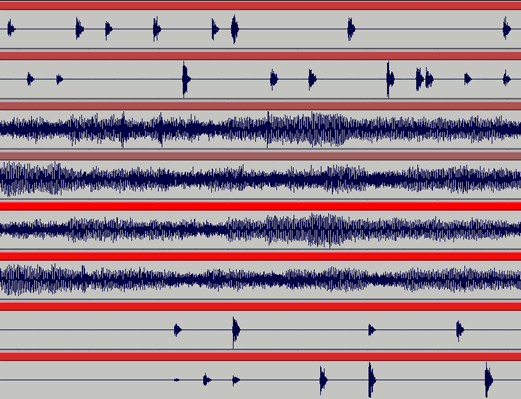
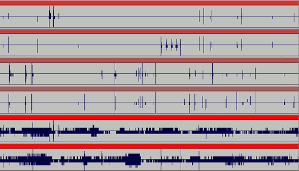
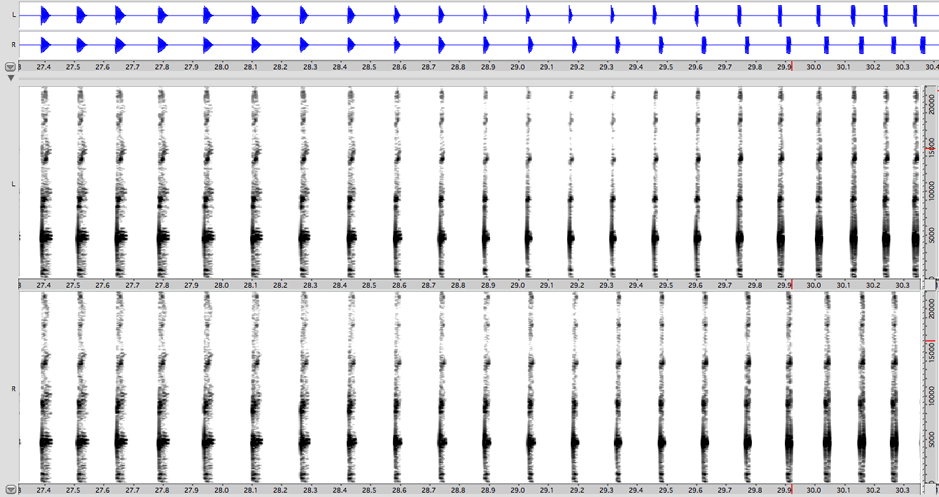
Here is an example of a ping-pong effect from my piece not even the rain (2000). [3] In this excerpt, two continuous stereo sounds are placed in the side speakers (channels 3–6) while short bursts “jump” independently from channel to channel. The position of each burst is very clear, while the rapid successions occasionally produce an impression of movement. (4)

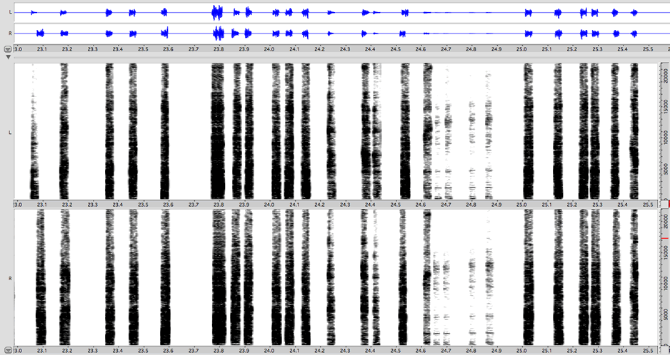
Here is a similar example from the piece brief candle (2005). [5] Each individual “insect” is clearly located in a specific speaker, while occasional quick movements are produced when they “sing” in rapid succession or when their voices overlap.

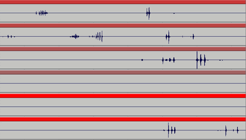
The third example is somewhat more complex, as many of the sounds are stereo (or two-channel) pairs. Thus the sounds may seem to be spread between the speakers, and the relations between the information on the two channels produces the perception of trajectories and complex movements. (This is discussed below in the section on decorrelation.)

Stream Segregation

The second result of fixed-channel routing is the perceptual segregation of different simultaneous auditory streams. When two sounds are produced by two different speakers, they are much more easily separated by the ear than when they are produced by the same speaker.

This is because of the way our brain processes the information it receives from our ears. The ears detect frequencies and amplitudes and send this information to the brain. The brain groups this information into auditory streams, so that instead of perceiving a single mass of frequencies we perceive separate sound sources: a voice, a piano, a bird. In order to do this, the brain uses various cues — one of which is spatial location. It is probable that all the frequencies that come from the same point in space are produced by the same physical source. (6)

Consider a noisy environment in which many people are speaking at once. How is it that we are able to separate out and follow the voice of a single speaker? It is partly because the voices of different speakers radiate from different points in space. Here is an audio example, prepared by John Pierce, of what is known as the “cocktail party effect.” In this example, two voices speak simultaneously: at first both are in the right speaker; then one is in the left speaker and the other in the right. Try to follow one of the voices; in which case is this easier? (7)

When two sounds come from the same speaker, the spatial cues indicate that they are produced by the same source (and in fact, they are: the speaker). If the sounds are different enough, we have no trouble separating them because the other cues tell us they are produced by different sources. But the more similar the sounds are, the harder this becomes.

In this example, both voices were recorded by the same person; we hear them as two voices, but we have trouble keeping them separated. If the example had been made with the voices of two different people, it would have been less difficult to maintain the separation. To demonstrate this, I have prepared a modified version of the example in which one of the two voices has been transposed down by a minor third. It is now possible to follow the two discourses independently even when they are produced by the same speaker.

On the other hand, if the two voices had been tied together in other ways besides spatial location, it would have been difficult not only to follow them independently but also to even perceive them as two separate sounds. Here is an example in which the two voices have been passed through a vocoder using identical parameters; thus they each produce the same frequencies. In the first part of the example, it is nearly impossible to distinguish two separate voices. In the second part, the separation is less clear than in the original example and this ambiguity produces some interesting spatial effects (again, see the section on decorrelation below).

Naturally, the importance of spatial location for auditory stream segregation is the same whether the information is linguistic or “musical.” Here is a final variation on the example from John Pierce; this time the two speaking voices have been replaced by two sawtooth oscillators wandering randomly in the same frequency range.

Clearly this phenomenon can change the musical meaning of the sounds. What follows is a stunning example from the CD Demonstrations of Auditory Scene Analysis, by Albert Bregman and Pierre Ahad. (8) In this track, two African xylophones play together; at first, each is panned to the centre, then they are gradually panned to the left and right speakers. In the beginning, when their spatial location is the same, we hear the rhythm that is produced by the fusion of the two lines; but as they are panned apart, this rhythm disappears and the two component rhythms (played by each of the instruments) emerge.

Thus it is quite clear that placing individual voices in different spatial locations helps to keep them perceptually distinct. This is one of the main reasons why I often compose in multi-channel formats, whatever spatialization techniques I may be using. However, because the spatial cues are clearest when the sounds are routed directly to individual speakers rather than panned between them, the greatest segregation of auditory streams is produced by fixed-channel routings without panning. This method allows the listener to follow the individual voices in complex polyphonic musics whose sounds might otherwise have a tendency to fuse into a dense mass.

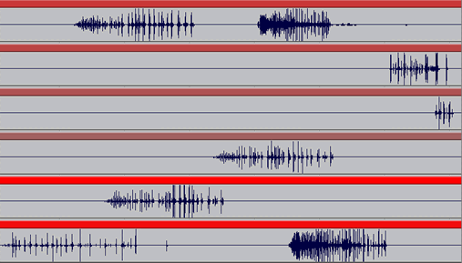
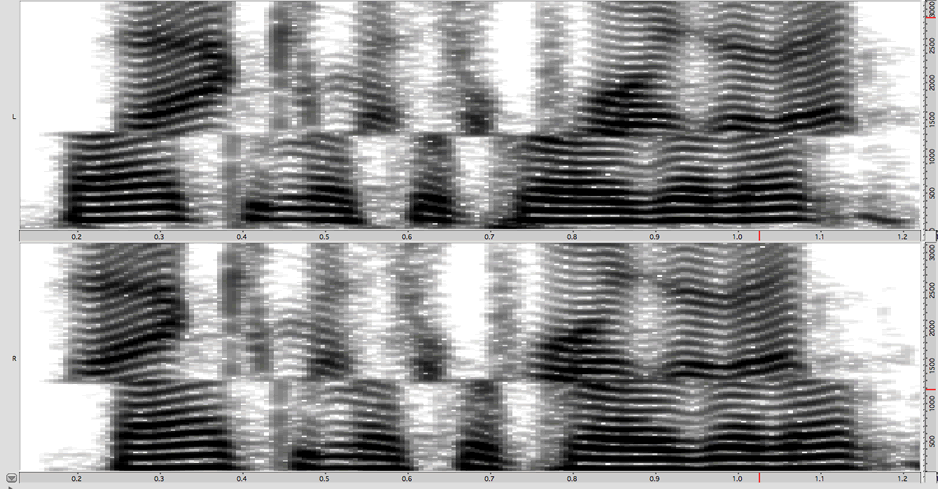
I will present now two examples from an eight-channel piece, 0.95652173913 (2005). [9] For this piece, the speakers are arranged as four left-right pairs surrounding the audience from front to back; the “spatialization technique” used was to place each two-channel sound in one of the four stereo pairs. The result is that each individual voice emerges clearly, even when the overall texture becomes extremely dense. (It is of course impossible to demonstrate this in stereo; see footnote 4 to download the full 8-channel versions.)

In stereo, we have little difficulty distinguishing the individual voices, and we can clearly hear the entrances of each of the sounds. However, in the multi-channel version, all the entrances are much clearer and the entire texture is much more transparent: rather than a mass, it is a tissue of interrelations.

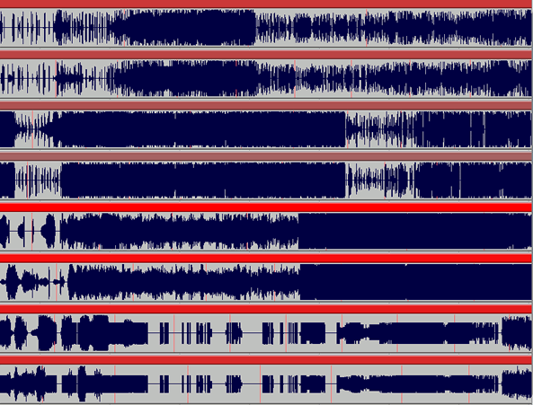
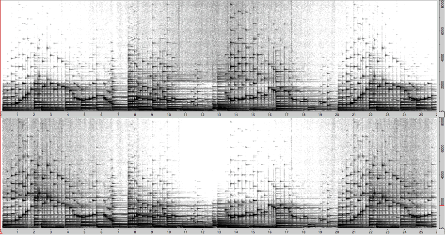
The second example is more extreme. The density of sound is extraordinary; in stereo, the result is something practically solid, like a rock. In the 8-channel version, on the other hand, we seem to be placed “inside” this density and are able to distinguish and to follow its individual component elements. The fact that the sounds are always placed in left-right pairs creates four planes of activity that remain relatively transparent or translucent to each other. We can focus our attention on one plane or another, listening to one plane “through” the others.

As these examples demonstrate, the simple fact of placing individual sound streams in different speakers produces a greater clarity, transparence and independence of voices; and this, in turn, permits the composer to work with a greater density of sonic “information.”

Decorrelation: Opening Up the Sound in Space

As I mentioned, each of the “voices” in the previous two examples is a 2-channel sound. There is a high level of spatial activity within each of these voices, and all of this activity is due to decorrelation: the differences between the information on the two channels.

The same is true of the second example from brief candle presented above (Audio example 3). Let us listen again to the end of that example, noticing the complex, rapid, rather random trajectories within the sound. (10)

This effect is similar to that produced by spatializer-type methods — except that what we hear is often something ambiguous between a single moving sound source and two or more sound sources emerging at different points in space. Here is a second example from the same piece. The sound is filled with active, complex spatial movements; in six channels, these trajectories are quite striking.

The Precedence Effect

Let us think again of a succession of two flashing lights. If the lights are positioned close together and the flashes follow one another in rapid succession, we may perceive one light that moves. If the lights are more widely separated or the flashes slower, we see two flashing lights. If they are in some intermediate relation, spatially or temporally, we may see something ambiguous between one and two. Such an ambiguity might also be produced if the flashes are somewhat different in colour, shape, size, intensity or some other parameter.

Similar phenomena occur in the two sound examples just presented. Yet the overall effect is much more complex, because there are many continually shifting relations among the sounds projected by the six speakers. As a result, different parts of the spectrum may appear in the speakers with different temporal relations, causing us to independently localize various elements of the sound.

These spatial effects result from the ways in which our brain processes auditory information. We have seen that rapid or overlapping ping-ponging produces the perception of movement. However, if the time difference is smaller (on the order of 5 to 50 ms.), rather than hearing two separate sounds or a single sound moving, we will hear one sound, localized at the position of the first source that reaches our ears. This phenomenon, known as the precedence effect, is very useful to us in understanding our environment. In a normal reverberant space, we are presented with the direct sound followed by hundreds of reflections. In determining the location of the sound source, our brain takes advantage of the fact that the direct sound usually reaches our ears first; it therefore pays particular attention to this first wave front and uses that information to localize the source. As the time difference is increased (above 50 ms. or so), the reflections emerge more and more clearly as independent sounds (echoes), located at the source of the reflection.

Thus, by simply altering the temporal relations between the channels of a 2-channel sound file, it is possible to modify the perceived location of the source and to perceptually divide the sound in two. What follows are four examples of the same sound file in which the temporal relations between the two channels shift gradually between two extremes. Here is how the delay times vary from the beginning to the end of the file:

As a result, at first the sound is localized to the right, then it gradually shifts to the left, and then back to the right. With each example the maximum delay time is increased: 6 ms., 12 ms., 30 ms., 60 ms. In the first example we hear a movement; as the delay times are increased, we hear the sound beginning to split in two; in the last example, the delayed channel is clearly audible as an echo (or independent source).

By simply separating the two channels of a stereo sound file, it is possible to produce various spatial effects: position, movement, envelopment, spaciousness, echo. I frequently use this simple technique when mixing, and I often have the impression that it opens up a spatial field within the sound itself rather than placing the sound-object in an external space.

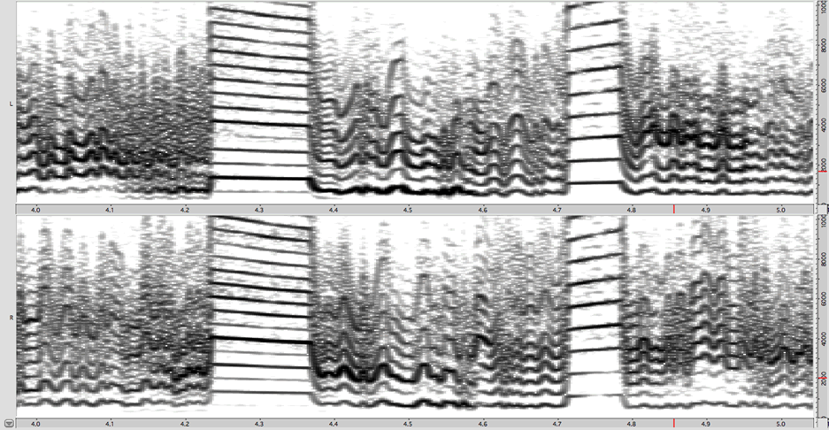
If the temporal difference is frequency-dependent — that is, if the delay times of separate spectral zones are altered independently — different components of the sound may be perceived as moving or splitting in independent ways. What follows are four more examples of the same sound file in which the timing of frequencies above 1200 Hz is shifted as above while those below 1200 Hz are shifted in the opposite direction. We hear the upper frequencies move from right to left to right while the lower frequencies move from left to right to left.

I next present four examples of the same technique applied to a piano sound, limiting myself to the first two delay times, 6 ms. and 12 ms. In Audio examples 21 and 22 the entire spectrum is shifted together; we hear the piano move from right to left to right. In Audio examples 23 and 24 the upper and lower frequencies are separated; we hear the notes of the piano spread between the speakers: at first, low-to-high notes are distributed from left to right, then they slowly reverse until they are spread from right to left, after which they slowly return to their “normal” positions.

What interests me here is not the production of a clear spatial perception of independent contrary movements of high and low frequencies. Even in these simple examples, we have to concentrate to hear these movements as such. However, we have an immediate and powerful — if difficult to define — “spatial” impression, which is the result of the independently shifting frequency zones. It is this spatial ambiguity itself that interests me. According to the spatial cues, the upper and lower frequencies arrive from different directions and therefore must belong to different sources; according to the other cues, all the frequencies are produced by a single speaking voice (or piano). The perceptual result is a strange and fascinating ambiguity regarding the spatial position and unitary identity of the sound.

Head-Related Transfer Function

The precedence effect is very important for spatial perceptions produced by time differences of roughly 5 to 50 ms. However, smaller differences can also have a major impact on our spatial perception.

The brain determines the position of sound sources by comparing the information that arrives at the two ears. Since sound takes time to travel through space, the fact that our ears are separated by about 17 cm means that all sounds except those originating directly in front, behind and above will arrive at the two ears at different times. These interaural time differences vary with the azimuth and elevation of the source; they are effective for the localization of frequencies up to about 1500 Hz. In addition, the head absorbs some of the energy of the sound, particularly at higher frequencies, and this absorption also varies with the position of the source. The resulting frequency-dependent interaural level differences are most effective for localizing frequencies above about 3000 Hz (the absorption is negligible below 500 Hz and ranges up to 20 dB above 5000 Hz).

It is possible to shift the perceived position of a sound by imitating these differences. The maximum interaural time difference (for sounds located 90° left or right) is very small: 0.69 ms. I find that in order to artificially create a clear perception of direction using only a small time difference between two audio channels, I need to exaggerate this difference substantially. Here are two examples, equivalent to Audio examples 13 and 17 above, in which the maximum time difference is 2.5 ms. This small timing variation results in a clear shifting of position. (11)

We can create a very crude imitation of head absorption by varying the relative levels of high frequencies in two audio channels. Here is an example, similar to Audio example 21 above, in which the amplitudes of the frequencies above 2000 Hz are varied by 24 dB. After filtering, the levels are adjusted to equal their pre-filtering level; thus any perceived movement is due only to the relative prominence of high frequencies in the two channels, not to any overall level differences.

Again, we hear the piano move from right to left to right.

Binaural techniques manipulate these interaural differences directly in order to produce the perception of localized sound sources for headphone listening. However, for creative compositional purposes and loudspeaker reproduction, it is possible to take advantage of these psychoacoustic phenomena, without necessarily seeking to produce a specific result. Since our brain is programmed to process slight time and level differences between the information received at the two ears, small differences in the information on separate audio channels have the potential to produce major perceptual spatial effects.

Conclusion and Examples

It should be clear by now that decorrelation techniques are difficult to control as such. Except in preparing the examples for this paper, I have rarely used them in order to obtain a specific result (such as simultaneously shifting upper and lower frequencies in opposite directions). However, striking — if often unforeseen — spatial effects are obtained by exploiting and exaggerating the differences between channels when processing or recording.

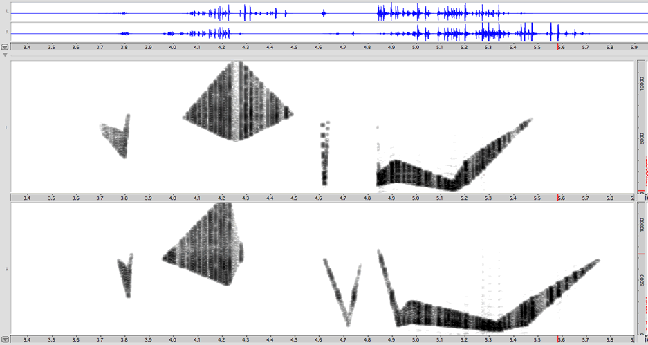
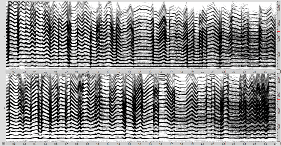
I will end with a few examples of two-channel sounds composed for brief candle and 0.95652173913. The processes used to create these sounds generate many rapidly-changing differences between the two channels. As a result of these differences — of timing, level, filtering, and frequency — the sounds have a rich and active “inner spatial life.”

Audio examples 28 and 29 below were produced using semi-random band-pass filters. In Audio examples 30 and 31, the sounds were processed by time-varying transposition. And in the final two examples, a sound fragment is read with constantly varying position, timing and speed. In each case, different but similar parameter values are generated for each channel.

The first example presents the same sounds twice: first mixed to mono and then separated left and right. When the channels are separated, the shifting relations between them produce a clear perception of rapid movements.

As the differences between the two channels become greater, what was perceived as a single sound source tends to divide into two. The following example is interesting in that we often hear the upper frequencies as a unified moving source while the lower frequencies are split into two separate sources.

The next example, produced by rapidly varying transposition, is ambiguous: the two channels are partly fused and partly separate.

In the following example, the differences are great enough that we clearly hear two sources; however, in a denser context they would be heard as one unit.

The next sound repeatedly shifts between being one and two: at times, we hear a single object at a specific location; at times, a single object moving, and at times two separate objects positioned left and right.

In the final example, the perceived object is again at times single, at times double, at times moving, at times fixed. The sound — sometimes mono, sometimes stereo — seems somehow to fill the space between the speakers.

Notes

1. See Chowning, Jot.
2. I am currently writing an article on the spit~ which will be published in 2010 in LIEN: L’espace du son III. http://www.musiques-recherches.be/edition.php?lng=fr&id=110
3. not even the rain was composed in the Métamorphoses d’Orphée studio (Brussels).
4. It is clearly impossible to demonstrate multi-channel spatial effects in stereo. The stereo sound examples in this article therefore are intended to give an idea of the result without necessarily reproducing it. Their effectiveness is variable. For those with the necessary equipment, the full set of multi-channel examples can be downloaded from the author’s website (AIFF, 44.1 kHz, 24 bit).
5. brief candle was commissioned by the French Ministry of Culture and by SCRIME (Bordeaux).
6. For a full discussion of the phenomenon of auditory stream segregation, see Bregman Auditory Scene Analysis.
7. John Pierce, “The Cocktail Party Effect.” Track 22 of the audio CD accompanying Music, Cognition, and Computerized Sound.
8. “Effects Of A Location Difference Of The Parts In African Xylophone Music.” From a recording by Ulrich Wegner, as presented in the following compact disc: Bregman, Albert and Pierre Ahad, Demonstrations of Auditory Scene Analysis, Track 41.
9. 0.95652173913 was commissioned by the French Ministry of Culture and by Ina/GRM.
10. The following two examples are only marginally effective in stereo.
11. Since I am here imitating the differences in the acoustic signals that actually excite the two eardrums, and since when using loudspeakers both ears receive the signal produced by each speaker, the following examples are most effective when listened to on headphones.

Bibliography

Bregman, Albert. Auditory Scene Analysis. Cambridge, MA: MIT Press, 1990.

Bregman, Albert and Pierre A. Ahad. Demonstrations of Auditory Scene Analysis. Audio CD. Department of Psychology, Auditory Perception Laboratory, McGill University, Montreal QC, Canada, 1996. http://webpages.mcgill.ca/staff/Group2/abregm1/web/downloadsdl.htm

Chowning, John. “The Simulation of Moving Sound Sources.” Journal of the Audio Engineering Society 19/1 (Winter 1971); pp. 2–6. (Also Computer Music Journal, June 1977, pp. 48–52.)

Jot , Jean-Marc. The Spat~ Processor and its Library of Max Objects: Introduction. Paris: Ircam, 1995.

_____. The Spat~ Processor and its Library of Max Objects: Reference. Paris: Ircam, 1995.

Pierce, John. “Hearing Sound in Space.” Music, Cognition, and Computerized Sound. Edited by Perry R. Cook. Cambridge MA: MIT Press, 1999.

Moore, Brian. “Space Perception.” An Introduction to the Psychology of Hearing. 4th ed. London: Academic Press, 1997, pp. 233–267.