Real-Time Spectral Analysis and Dispersion

by Martin Ritter

This paper was originally presented at the Toronto Electroacoustic Symposium 2008 (7–9 August 2008).

Abstract

A software implementation of a Real-Time Spectral Analysis and Dispersion tool (or Real-SAD) using the Max/MSP programming environment is described. Real-SAD allows the user to analyze, resynthesize, and distribute the individual spectral components in a multichannel environment in real time.

1. Introduction

The Real-SAD tool was developed for real-time sound analysis and manipulation in a concert setting using sensor interfaces such as the Teabox with the Max/MSP programming environment (1). The motivation for this development was a desire to discover and explore a timbre’s various spectral components in real-time and disperse them throughout a multichannel environment in concert. Real-SAD allows the user to play a sound forwards or backwards at various speeds, and surround listeners with the timbre rather than presenting the summed components from a single point source.

2. General Description

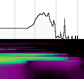
Real-SAD consists of three bpatchers (bp) that handle the recording, analysis, resynthesis and distribution of a timbre. It also has a control structure for managing volume and smoothing factors, as well as spectral displays for showing the data in the amplitude-frequency and the frequency-time domain using spectroscopes (Fig. 1).

In bp1 — the “fft-scrubber” — the recording, analysis, distribution and re-synthesis of audio material are carried out. bp2 gives the user intimate control over the bin-wise reconstruction and deconstruction of the analyzed material, while bp3 distributes the output of bp1 in an eight-channel environment. Each bpatcher will be discussed in detail in the following sections.

3. BPatchers

3.1 bp1: FFT-Scrubber

The FFT-Scrubber is used for recording and loading libraries of sound clips and then performing the real time spectral analysis and diffusion. Much of the implementation of the recording portion of it was taken from the Cycling 74 “MSP Tutorials and Topics, Tutorial 26” (2). This information was supplemented and expanded upon with the help and knowledge of various people from the Cycling 74 Max/MSP forum (3).

3.1.1 Initial Analysis and Recording

After analyzing the sample using a Fast Fourier Transform (FFT) the pfft~ subpatch stores the resulting data in a buffer for further processing. However, before the data can be written, it has to be converted from Cartesian coordinates to Polar coordinates. This avoids the necessity of using complex math to analyze and manipulate the data. In order to achieve this the real and imaginary numbers from the fftin~ (left and middle outlets) are sent through the cartopol~ object to be converted to amplitude and phase pairs. The amplitude is stored in channel 1 of the buffer~ analysisAll, while the phase information is sent through the framedelta~ and phasewrap~ objects. framedelta~ computes the phase difference or deviation between consecutive frames of data, and phasewrap~ ensures that the data is properly constrained between -π and π. The phase difference is then stored in channel 2 of buffer~ analysisAll. Using this initial analysis, the rest of the “scrubber”-related patch is able to extract and re-synthesize the spectral components.

3.1.2 Initial Data Acquisition

In Real-SAD each FFT frame has 512 bins per data type (amplitude and phase). In order to access this data at any location within the buffer, the index~ object is used and it needs to process all of the data within a frame before moving on to the next. To accomplish this the sah~ (sample and hold) object collects the data from the mother patch and holds it until all 512 bins have been obtained and processed. Once that has occurred it begins to accept new frame data.

The right outlet of fftin~ is used to synchronize this operation. This outlet creates samples matching the current frame of data in the order of 0 to (frame size -1). By feeding the right outlet of fftin~ into the left inlet of the +~ object and feeding the output of sah~ to the right inlet of +~, it is assured that the re-synthesis will have 512 bins of information per frame. One issue that arises is that the user may not read through the buffer incrementally. In order to allow this, frameaccum~ is used to change the phase deviation to a running phase value, allowing for non-incremental parsing of the buffer data.

The data can now be passed through the poltocar~ object which converts the data back to real and imaginary numbers (that is, from Polar coordinates back to Cartesian coordinates) and then sent through an fftout~ object for re-synthesis. At this point a simple phase vocoder has been constructed (4–10).

3.1.3 Bin Sorting and Playback

The second major component to the pfft~ subpatch is the index sorting and playback routine, which consists of two major parts described below. All subpatches in this part have the ability to receive the control data from bp2 via the spray 64 object, which receives a location and index pair. The pair is parsed by spray 64 sending the index to the specified location to be retrieved by fmt.mess sending out the associated amplitude (see 3.1.3.2 below).

3.1.3.1 Bin Sorting

In order to correctly sort the indices and corresponding amplitude information, it is necessary to write that information into a new buffer called buffer~ amp. Rather than using record~ as in section 3.1.1, poke~ is used for its ability to index the incoming data at specific points in the buffer. By connecting the synchronization outlet of fftin~ to poke~ amp the incoming data will always be found in buffer position 0 through 511. Because of this, the peek~ object can be used to transfer the data from buffer~ amp into a list for storage. For this purpose IRCAM’s fmat (11) was chosen for its faster access and manipulation times as well as the ability to hold larger sets of data.

Once the data is transferred from the buffer to the fmat object, the column containing the amplitude data is reordered from highest to lowest.

3.1.3.2 Bin Playback

Real-SAD is able to play back up to sixty-four individual bins for eight different outputs. This is achieved in the binPlayback subpatches. Once the fmat object has reordered the bins the fmt.mess objects inside binPlayback access this information according to the selections from bp2. The corresponding amplitude information is sent into the right inlets of ==~ whose left inlets are connected to the output of index~ 1 analysisAll. The data from each bin passes through a gate~ object controlled by an ==~ object. If the bin amplitude data is equal to the selected amplitudes (as chosen using the Bin Selector), the gate is opened and the corresponding amplitude and phase information is sent through to be resynthesized.

After the filtered signal is sent through a poltocar~ object, it arrives at vectral~ which is a vector-based envelope follower. Connected to the right outlet of fftin~ for synchronization, the vectral~ object allows the user to smooth any changes in bin values between frames. The smoothing can be achieved in three different ways: linearly over n frames via the message rampsmooth int int, logarithmically via slide float float, or simply by limiting the amount of change allowed via deltaclip float float (where 0 means no changes are allowed). The last smoothing method defined by the separate control structure is the current mode of operations (rampsmooth is the default method). Following this fftout~ resynthesizes the data and sends it out eight different outputs for diffusion.

3.2 bp2: Bin Selector

In order to give the user maximum flexibility over the sculpting of the sound, the Bin Selector was created. It consists of two jit.cellblock objects, one keeping track of the index number and the other checking the On/Off or active status of each cell.

By default, the first sixty-four indices are visible, although by scrolling down all 511 indices are accessible if desired. If higher numbered indices are selected the Main Volume will have to be increased in order to clearly hear those bins. For that purpose the Main Volume slider has been designed in such a way that the slider is open-ended. When the high value of the slider is changed, the current output level is held at its current position. If the new high value is below the current output, the output will be scaled to the new high.

In an eight-speaker setup each column of the jit.cellblock corresponds to one speaker, with a maximum output of eight bins per speaker (8x8 —> 64 bins). The “active bins” counter on the bottom of bp2 indicates how many cells in any given column are currently set to On. Only eight simultaneous bins are possible per channel; if the “active bins” number is greater than this, the binPlayback subpatch in bp1 wraps around and turns off earlier bins as needed. Currently the wrap-around only happens internally in bp1, which means the jit.cellblock does not display these changes by deselecting these cells.

Further customizations of the cellblock are possible: all OFF resets all cells to off, regardless of offset; all visible On turns on all visible cells, keeping track of the offset; randomize turns cells on and off randomly, also keeping track of the offset as well as keeping track of which columns have been designated for randomization via the check boxes. The number box sets the random speed in milliseconds; cellblock offset displays the current offset when jit.cellblock itself is used for scrolling through the indices and may also be used to change said offset as well; range of columns allows for quick changes in column assignment for use with the random function.

3.3 bp3: Diffusion

For diffusion the Ambisonics Tools for Max/MSP by ICST (12) are used. These tools allow for quick changes in speaker configurations (two preset configurations are provided and can be changed on the fly), and provide a great deal of freedom in the movement of sound. Two displays representing the sound field give information about sound location and movement and also provide a control interface.

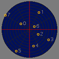
In Display No.1 each incoming channel is assigned a number from zero to seven. These numbers match the jit.cellblock numbering and appear in the sound field representation in a box. Within the box the source moves about randomly, resulting in a slightly localized movement of the source. This movement provides greater interest for listeners as the sound sources are never static in their positioning. The size of the box is user-definable, allowing for a greater or lesser degree of random positioning in that area of the sound field, terminating any movement if set to 0.

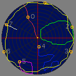
Display no. 2 allows the user to control the overall movement of the sound around the sonic field. The user can manually move each sound around the soundfield by clicking and dragging or else by letting the computer randomize and/or rotate the sound.

The use of trajectories is another feature of the Ambisonics Toolbox. One trajectory preset is provided, which can be turned On/Off via the traj.OnOff button. The preset will move each source from its individual speaker location to the center of the sonic field and back, in a continuous loop. The speed of the trajectory can be manipulated using the traj.Speed number box, where 1 is the original speed, 2 will be double speed, etc. Trajectories can also be customized. When the custom button is turned on, the user may click, hold and drag any point. While the mouse-button remains held, the movement of the point within the display will be recorded. Once the button is released the custom trajectory will be executed. Each point (0–7) may have its own trajectory and the trajectories may be changed at any time, as long as custom is still set to On. The traj.Speed may be altered as well. Note, however, that the random and rotate features will not work with customized trajectories.

Any trajectory may be saved with the read and write messages. One .xml file with break-point functions will be created for each point and subsequently read. reset will change all points to their original position according to the chosen speaker configuration and erase all customized information with the preset trajectory.

4. Future Work

Currently the initial recording section of bp1 does not facilitate real time input. However, it is expected that by using several interlocking buffers it would be possible to achieve actual real-time input/output. As well, mapping strategies for intuitively changing the spectral characteristics (e.g. mapping the x loudest amplitudes to the x softest frequencies) will be explored.

The Real-SAD tool was originally conceived and developed for in-concert use. To this end CPU usage is a constant concern. Future developments will include increasing CPU efficiency so that multiple sets may be run from a single computer and polyphonic voicing made possible. For non-real time uses of Real-SAD (e.g. for source sound creation for electroacoustic compositions, or other interactive pieces) an intuitive and adaptable recording interface will be added. Currently a toolset is in development for smoothing and scaling incoming sensor-data in accordance with the specifications of bp1.

5. Conclusion

A toolkit for real-time spectral analysis and dispersion has been created which allows the user a maximum amount of freedom for manipulation of the source material’s spectrum. Currently, any 64 of 512 bins per frame may be accessed and output in an adaptable and user driven 8-channel ambisonic environment. The source material may be played back at any speed, forward or backward and several options are available for smoothing differences between successive frames.

6. References

1. http://www.cycling74.com
2. Dobrian, Christopher et al. “MSP Tutorials and Topics.” Version 4.6, pp. 201–19, 2006.
3. http://www.cycling74.com/forums
4. Dudas, Richard and Corte Lippe. “The Phase Vocoder — Part I.” http://www.cycling74.com/story/2006/11/2/113327/823.
5. _____. “The Phase Vocoder — Part II.” http://www.cycling74.com/story/2007/7/2/112051/0719
6. Dolson, Mark. “The Phase-Vocoder: A Tutorial.” Computer Music Journal 10/4 (1986), pp. 14–27.
7. Flanagan, James L. and R.M. Golden. “The Phase Vocoder.” The Bell System Technical Journal 45 (1966), pp. 1493–1509.
8. Laroche, Jean and Mark Dolson.”New Phase-Vocoder Techniques For Pitch-Shifting, Harmonizing and other Exotic Effects.” Proceedings of the IEEE Workshop on Applications of Signal Processing to Audio and Acoustics 1999, pp. 91–94.
9. Fishman, Rajmil. “The Phase Vocoder: Theory and Practice.” Organised Sound 2/2 (1997), pp. 127–45.
10. Prerau, Michael J. “Slow Motion Sound: Implementing Time Expansion/Compression with a Phase Vocoder.” http://www.music.columbia.edu/~mike/publications/ PhaseVocoder.pdf
11. http://ftm.ircam.fr/index.php/Main_Page
12. http://www.icst.net/downloads